CICI
CICI is an package for Causal Inference with Continuous Interventions.
It facilitates estimation of counterfactual outcomes for multiple values of continuous interventions at different time points, and allows plotting of causal dose-response curves (CDRC). It can address positivity violations through weight functions.
The package implements the methods described in Schomaker, McIlleron, Denti and Díaz (2023), see here. It can be used for non-continuous interventions too. Briefly, the paper describes two approaches: the first one is to use standard parametric $g$-computation, where one intervenes on multiple values of the continuous intervention, at each time point. This approach may be complemented with diagnostics to understand the severity of positivity violations. An alternative approach is to use sequential $g$-computation where outcome weights redefine the estimand in regions of low support. Note that developing $g-$formula-based approaches for continuous longitudinal interventions is an obvious suggestion because developing a standard doubly robust estimator, e.g. a TMLE, is not possible as the CDRC is not a pathwise-differentiable parameter; and developing non-standard doubly robust estimators is not straightforward in a multiple time-point setting.
$\rightarrow$ standard parametric $g$-formula
$\rightarrow$ weighted sequential $g$-formula
Installation
The package is available on CRAN. The weighted sequential approach is currently only available on GitHub and needs to be installed seperately, but will be integrated into the main package later:
install.packages("CICI")
library(remotes)
remotes::install_github("MichaelSchomaker/CICIplus")
Standard $g$-computation for continuous interventions
Standard application
As an example, consider the efavirenz data contained in the package. This simulated data set is similar to the real data set described in Schomaker et al. (2023; see paper on more details, including identification considerations). We are interested in what the probability of viral failure (binary outcome) at time $t$ would be if the concentration was $a$ mg/l for everyone ($a=0,…,10$), at each time point. If the intervention values do not change over time, we can simply specify a vector under $\texttt{abar}$ that contains the values with which we want to intervene. Apart from this, only the dataset ($\texttt{X}$), time-varying confounders ($\texttt{Lnodes}$), outcome variables ($\texttt{Ynodes}$) and intervention variables ($\texttt{Anodes}$) need to be specifed. Baseline variables are detected automatically:
library(CICI)
data(EFV)

# parametric g-formula
est <- gformula(X=EFV,
                Lnodes  = c("adherence.1","weight.1",
                            "adherence.2","weight.2",
                            "adherence.3","weight.3",
                            "adherence.4","weight.4"),
                Ynodes  = c("VL.0","VL.1","VL.2","VL.3","VL.4"),
                Anodes  = c("efv.0","efv.1","efv.2","efv.3","efv.4"),
                abar=seq(0,10,1)
)

est        # print estimates
plot(est)  # plot estimates
The $\texttt{plot}$ functionality can be used to plot the estimated counterfactual outcomes in terms of dose-response curves at different time points. In the below example, the curve at $t=5$ means that we look at $Y_5 = \text{VL}.4$ under the interventions $(0,0,0,0,0),…,(10,10,10,10,10)$:
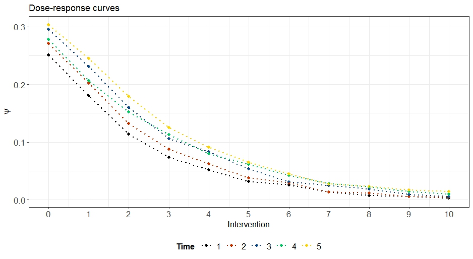
More complex custom interventions that change over time can be specified too under $\texttt{abar}$, and they will be plotted differently; type $\texttt{?gformula}$ for details.
Bootstrap confidence intervals
To obtain bootstrap confidence intervals, simply specify the number of bootstrap samples in the option $\texttt{B}$. CI’s can also be plotted. Examples are given in the example code listed further below (parallelization using the option $\texttt{ncores}$ is recommended).
Other estimands
In $\texttt{CICI}$, it is easy to estimate and plot other estimands than $E(Y^{abar})$. Simply, i) set the option $\texttt{ret=T}$ in $\texttt{gformula()}$, which saves the counterfactual datasets under the different interventions; and then, ii) apply the integrated $\texttt{custom.measure}$ function:
custom.measure(est, fun=prop, categ=1) # P(Y^a=1) - > identical results
custom.measure(est, fun=prop, categ=0) # P(Y^a=0)
custom.measure(est, fun=prop, categ=0, cond="sex==1") # conditional on sex=1

# does not make sense here, just for illustration:
custom.measure(est, fun=quantile, probs=0.1) # counterfactual quantiles
Model specification
The longitudinal parametric $g$-formula requires fitting of both confounder and outcome models at each time point. By default (as a starting point) GLM’s with all variables included are used, though CICI is implemented in a more general and flexible GAM framework. The model families are picked by $\texttt{CICI}$ automatically and are restricted to those available within the $\texttt{mgcv}$ package to fit generalized additive models. As correct model specification is imperative for the success of $g$-formula type of approaches, variable screening and the inclusion of non-linear and interaction terms is often important. The package comes with built-in wrappers to help with this. A recommended approach is to start as follows: 1) generate (strings of) all relevant model formulae with the function $\texttt{make.model.formulas}$, then 2) screen variables with LASSO using $\texttt{model.formulas.update}$ and then 3) pass on the updated formulae (possibly aftr furthr manual updates, see below) to $\texttt{gformula}$ using the $\texttt{Yform, Lform, Aform, Cform}$ options, as required by the estimand.
# 1) Generic model formulas
m <- make.model.formulas(X=EFV,
                         Lnodes  = c("adherence.1","weight.1",
                                     "adherence.2","weight.2",
                                     "adherence.3","weight.3",
                                     "adherence.4","weight.4"),
                         Ynodes  = c("VL.0","VL.1","VL.2","VL.3","VL.4"),
                         Anodes  = c("efv.0","efv.1","efv.2","efv.3","efv.4")
)
m$model.names # all models potentially relevant for gformula(), given *full* past

# 2) Update model formulas (automated): screening with LASSO
glmnet.formulas <-  model.formulas.update(m$model.names, EFV)

# 3) use these models in gformula()
est <- gformula(...,
                Yform=glmnet.formulas$Ynames, Lform=glmnet.formulas$Lnames,
                ...)
Obviously, even with this approach one may have to still manually improve the models, for example by adding (penalized) splines and interactions. Examples are given at the bottom of the following help pages: $\texttt{?fit.updated.formulas, ?model.update}$. A future manual will give more details on possibilities of model specification.
Multiple imputation
CICI can deal with multiply imputed data. Currently the option MI Boot, explained in the publication further below (Schomaker and Heumann, 2018), is implemented. Simply use $\texttt{gformula}$ on each imputed data set and then use the $\texttt{mi.boot}$ command (custom estimands are possible too after imputation):
# suppose the following subsets were actually multiply imputed data (M=2)
EFV_1 <- EFV[1:2500,]
EFV_2 <- EFV[2501:5000,]

# first: conduct analysis on each imputed data set. Set ret=T.
m1 <- gformula(..., ret=T)
m2 <- gformula(..., ret=T)

# second: combine results
m_imp <- mi.boot(list(m1,m2), mean) # uses MI rules & returns 'gformula' object
plot(m_imp)

# custom estimand: evaluate probability of suppression (Y=0), among females
m_imp2 <- mi.boot(list(m1,m2), prop, categ=0, cond="sex==1")
Other useful options
There are many more useful option, wich are explained in $\texttt{?gformula}$:
- How to handle survival settings
- How to generate diagnostics
- How to specify both custom and natural interventions
- Parallelization using the option $\texttt{ncores}$ (very easy!)
- How to track progress, even under parallelizations with $\texttt{prog}$
- How to reproduce results using $\texttt{seed}$
The package can of course also handle binary and categorical interventions. Dynamic interventions are not supported.
Weighted sequential $g$-computation
Basic (unweighted) setup
The function $\texttt{sgf()}$ implements the sequential $g$-formula and works very similar as $\texttt{gformula()}$. The below example illustrates this. The estimated CDRC’s are very similar.
library(CICIplus)

# (unweighted) sequential g-formula
est2 <- sgf(X=EFV,
            Lnodes  = c("adherence.1","weight.1",
                        "adherence.2","weight.2",
                        "adherence.3","weight.3",
                        "adherence.4","weight.4"),
            Ynodes  = c("VL.0","VL.1","VL.2","VL.3","VL.4"),
            Anodes  = c("efv.0","efv.1","efv.2","efv.3","efv.4"),
            abar=seq(0,10,1)
)
est2
plot(est2)
Calculating outcome weights
The function $\texttt{calc.weights}$ calculates the outcome weights described in equation (12) of Schomaker et al. (2023). The setup is simple: i) define variables as confounders, outcomes, interventions or censoring indicators; ii) choose a method for conditional density estimation, iii) specify one or many values for $c$, to specify how low support regions are defined:
# Step 1: calculate weights (add baseline variables to Lnodes)
# a) parametric density based
w <- calc.weights(X=EFV,
                         Lnodes  = c("sex", "metabolic", "log_age",
                                     "NRTI" ,"weight.0",
                                     "adherence.1","weight.1",
                                     "adherence.2","weight.2",
                                     "adherence.3","weight.3",
                                     "adherence.4","weight.4"),
                         Ynodes  = c("VL.0","VL.1","VL.2","VL.3","VL.4"),
                         Anodes  = c("efv.0","efv.1","efv.2","efv.3","efv.4"),
                         d.method="binning", abar=seq(0,10,1),
                         c=c(0.01,0.001)
)
summary(w) # weight summary
# d.method alternatives: parametric density estimation or highly-adaptive LASSO based
# check ?calc.weights for details
Weighted sequential $g$-formula
We can now use the calculated weights in the sequential $g$-formula by using the $\texttt{Yweights}$ option. The estimation algorithm is listed in Table 1 of Schomaker et al. (2023):
# Step 2: sequential g-formula with outcome weights
est3 <- sgf(X=EFV,
              Lnodes  = c("adherence.1","weight.1",
                          "adherence.2","weight.2",
                          "adherence.3","weight.3",
                          "adherence.4","weight.4"),
              Ynodes  = c("VL.0","VL.1","VL.2","VL.3","VL.4"),
              Anodes  = c("efv.0","efv.1","efv.2","efv.3","efv.4"),
              Yweights = w$`0.01`,
              abar=seq(0,10,1)
)
Super Learning
The sequential $g$-formula needs models for the iterated nested conditional outcomes. In the case of binary outcome variables (and more than 1 time point) this equates to modeling proportional data as of the second iteration step. Using a data-adaptive approach, with super learning, is thus a good option. Candidate learners, and screening algorithms, can be easily passed on to the $\texttt{SuperLearner}$ package. Note that user-written learners (as in the example below) need to be listed in the option $\texttt{SL.export}$ if parallelization is used (thanks to Eric Polley for helping me here!).
# Realistic setup
# (requires user-written learners which are available upon request)

library(SuperLearner)
est5 <- sgf(X=EFV,
            Lnodes  = c("adherence.1","weight.1",
                        "adherence.2","weight.2",
                        "adherence.3","weight.3",
                        "adherence.4","weight.4"),
            Ynodes  = c("VL.0","VL.1","VL.2","VL.3","VL.4"),
            Anodes  = c("efv.0","efv.1","efv.2","efv.3","efv.4"),
            Yweights = w$`0.01`,
            SL.library = list(c("SL.glm","screen.glmnet_nVar_1_4_10_150"),
                              c("SL.mgcv_base", "screen.cramersv_3")),
            SL.export = c("SL.mgcv_base","screen.glmnet_nVar_base",
                          "screen.cramersv_base","predict.SL.mgcv"),
            abar=seq(0,10,1), B=200, ncores=7, seed=41188, prog="C:/temp",
            cvControl = list(V=2), # SL option
            calc.support=TRUE
)
est5                                    # estimates
est5$SL.weights                         # Super Learner summary
plot(est5, time.points = c(1,5), CI=T)  # plot with CIs
Further options
The weighted sequential $g$-formula approach can also handle survival settings. There are many important subtleties related to the estimation of the conditional densities needed to calculate the outcome weights. It is possible to customize density estimation with the highly-adaptive LASSO, and pass on many useful options; details will be described in the future manual.
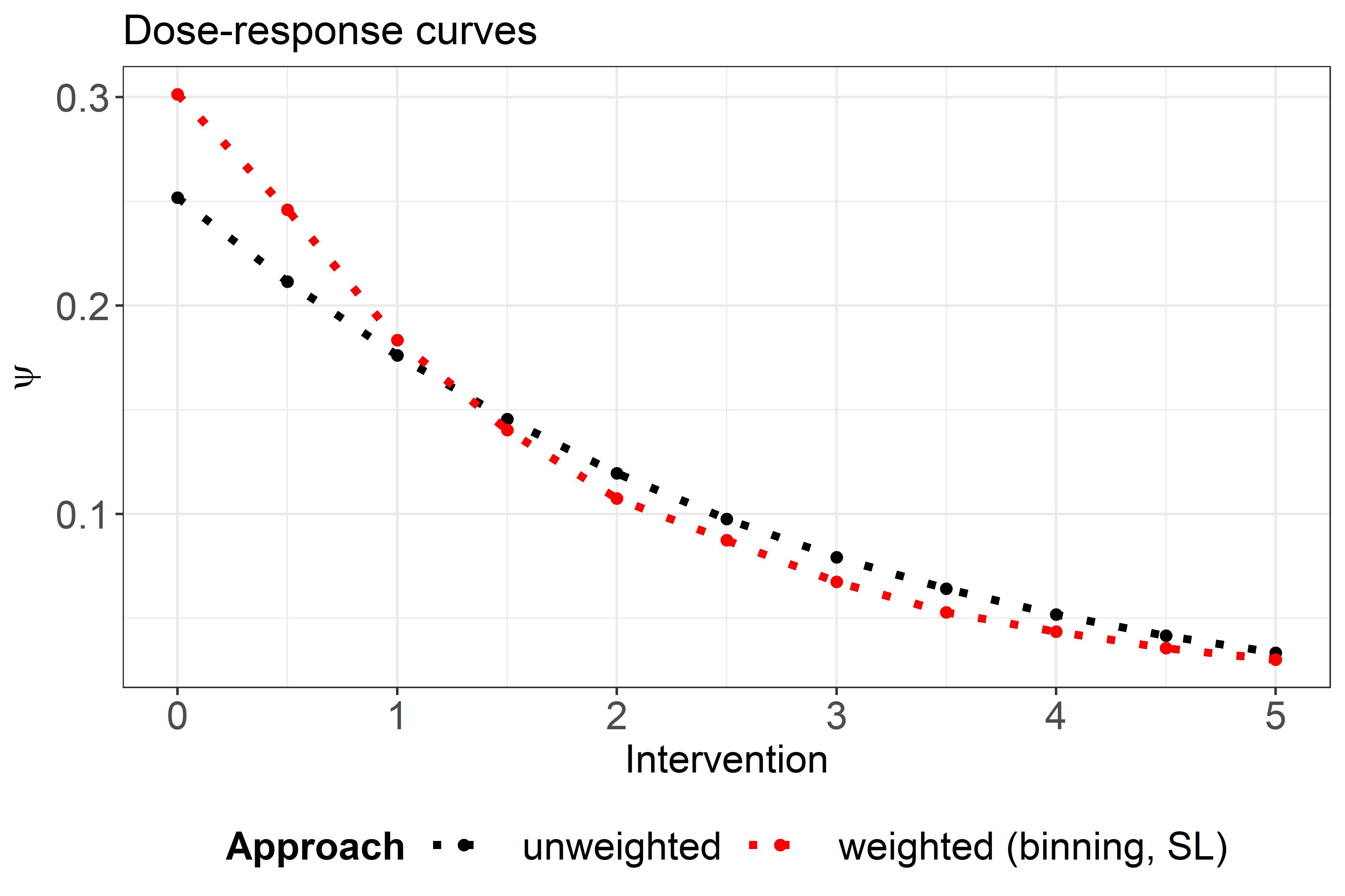
Comparison
As a comparsion between the standard and weighted approach have a look at the below figure: in areas of low support (close to 0), the weighted curve is different, but otherwise similar. Details about the interpretation of the weighted curve can be found at the bottom of Section 3.2.2 in the paper.
Code
The code of this little tutorial is available here.
Publications
Bootstrap inference when using multiple imputation